Continuous Blackjack

Everyone's heard of Blackjack, but I'd hazard a guess that you've not heard of Continuous Blackjack. I hadn't either until a short while ago, but something about the game captured my attention. In the traditional setting, each player draws cards from a deck until they choose to stick on a given hand. The goal is simple: finish with the highest hand without exceeding 21. There are of course many game theoretic considerations to this — strategy plays a key role — but the actual mechanics are pretty straightforward. The continuous variant of the game shakes this up: rather than draw cards with discrete values between 1 and 11, you now draw values from some continuous distribution; in our case a uniform distribution on \([0, 1]\). The premise is otherwise unchanged: you aim to get the largest hand without exceeding some upper threshold, be it 21, \(\pi\), \(e\), or some other value.

The problem itself is easy to explain and understand, but I wanted to dive a bit deeper. After a little bit of analysis, it became clear that the problem was surprisingly rich in theory. What's more, there are some nice subtleties that can lead you astray if you're not careful, making it particularly juicy. I felt compelled to share and, thus, Regular Dose was born. In this article, to keep things short, we will only cover the basic modelling aspects of the problem; in the next article we'll address the multi-agent elements and take into account the strategy involved in a more realistic setting. So for anyone reading, I hope you enjoy! There will be more to come.

Hands and their Distributions

The first thing we need is a model for our current hand: that is, the sum of all our draws up until the current time. For this, we introduce a discrete-time stochastic process \(S_n \doteq \sum_{k=1}^n X_k\), \(n \geq 1\), whose values are the \(n\)-fold summations of an independent and identically distributed (IID) sequence of uniform random variables \(\{X_n \sim \mathcal{U}(0, 1) : n \geq 1\}\). One can thus interpret the process \(\boldsymbol{S} = S_1, S_2, S_3, \dots\) as a cumulative sum over the various draws — i.e. our current hand — with both stationary and independent increments. Note that the IID assumption will be necessary in our analysis, but one could certainly relax this to cases where \(\boldsymbol{X}\) is appropriately adapted.^[a]

Now, since \(\boldsymbol{X}\) has uniform marginals, we can appeal to the Irwin-Hall distribution^[1] to describe the probabilistic behaviour of \(S_n\) for \(n \geq 1\). Defining the function $$\alpha_n^m(s) \doteq \frac{1}{m!} \sum_{k=0}^{n} \binom{n}{k} (-1)^k \mathrm{sign}(s - k) (s - k)^m,$$ we can show (with some abuse of notation) that the cumulative distribution function (CDF) is given by $$\alpha_n(s) \doteq P(S_n \leq s) = \frac{1 + \alpha_n^n(s)}{2}$$ and thus that the probability density function (PDF) is $$\dot\alpha_n(s) \doteq P(S_n = s) = \frac{\alpha_n^{n-1}(s)}{2}.$$ We omit the derivation of these quantities as they're well known, but note that the function \(\alpha_n^m(s)\) has some particularly nice properties! For example, taking the derivative with respect to \(s\) has the effect of decrementing the integer variable \(m\): \(\nabla_s \alpha_n^m(s) = \alpha_n^{m-1}(s)\). Conversely, integrating the function \(s \mapsto \alpha_n^m(s)\) increments the value of \(m\) by one, yielding the convenient relationship that \(\int \alpha_n^m(s) \, \mathrm{d}s = \alpha_n^{m+1}(s) + C\). These all translate naturally to the marginal CDFs and PDFs of \(\boldsymbol{S}\), and will feature later.

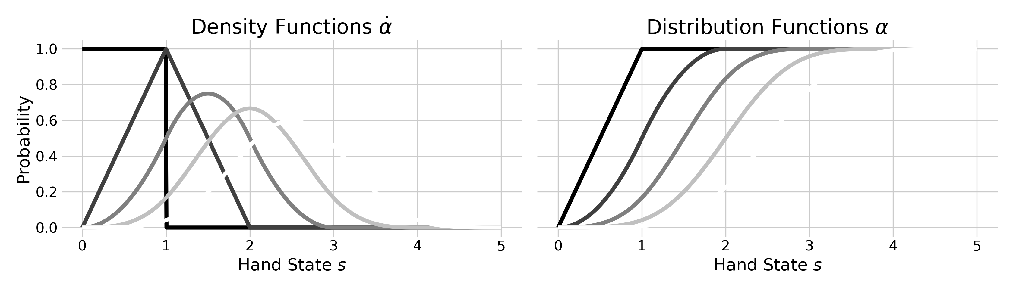
It is worth noting at this point that both \(\alpha\) and \(\dot\alpha\) have piecewise functional forms for small \(n\), as illustrated above. While \(S_n\) tends towards a Normal distribution as \(n\to\infty\), the behaviour for \(n \in \{1, 2\}\) will turn out to be absolutely crucial in our later analysis involving CDF queries that lie outside the unit interval.

Stopping Times and Strategies

As outlined in the problem statement, our goal is to stop/stick just before some upper limit which we'll denote by \(\theta\). Go too high and risk going bust and losing our stake; go too low and we decrease our competitive advantage, more than likely losing our stake. The challenge lies in identifying an appropriate condition on our current hand such that the corresponding probability of success, or expected payoff, is greatest. We'll tackle this problem by considering a strategy that is parameterised by a threshold \(\tau \in [0, \theta)\) over which we stop drawing new samples. This formulation is justified by the intermediate value theorem^[3] and lends itself well to renewal theory and all the machinery that comes with it. In the following paragraphs we'll explore a formal characterisation of its properties.

Let \(N(s) \doteq \max_{n \geq 0}\{ n : S_n \leq s \}\) denote the number of draws prior to the threshold \(s \geq 0\). This (continuous-time) stochastic process is referred to as the renewal counting process associated with interarrival sequence \(\boldsymbol{X}\), and is a generalisation of the Poisson process to arbitrary jump distributions; in this case, uniform. Of particular interest in our case is the stopping time \(N(\tau) + 1\) which describes the number of jumps/draws required to exceed \(\tau\) and (ideally) land in the region \((\tau, \theta]\). A foundational property of renewal processes — namely, that the events \(\{N(s) \geq n\}\) and \(\{S_n \leq s\}\) are equivalent (see below) — allows us to reason about these quantities by appealing only to the distributional nature of \(\boldsymbol{S}\).

For brevity, define \(\beta_s(n) \doteq P(N(s) \leq n)\) and \(\dot\beta_s(n) \doteq P(N(s) = n)\) to be the CDF and probability mass function (PMF) of the renewal counting process at threshold \(s\), respectively. To derive closed-forms for \(\beta\) and \(\dot\beta\) we need only appeal to the event equivalency principle which states that \(P(N(s) \leq n) = P(N(s) < n + 1) = P(S_{n+1} > s) = 1 - P(S_{n+1} \leq s)\). In other words, the CDF is given by $$\beta_s(n) = 1 - \alpha_{n+1}(s)$$ and the PMF by $$\dot\beta_s(n) = \alpha_n(s) - \alpha_{n+1}(s).$$ Note that \(\alpha_n\) and \(\beta_s\) have reversed notation with regards to the subscript and arguments in order to maintain the traditional semantic meaning of a CDF/PDF/PMF.

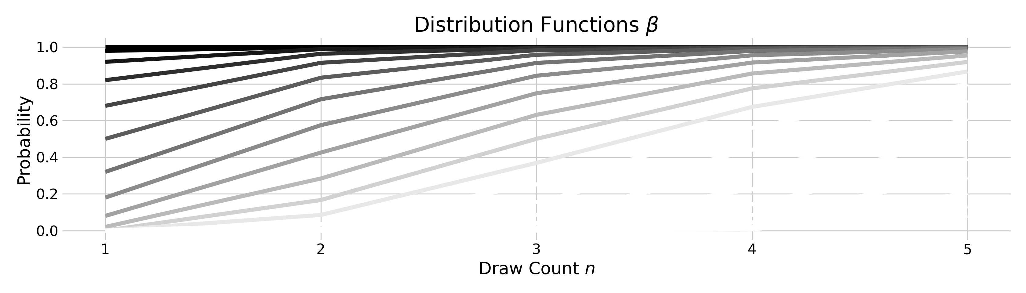
Great! Now we've now captured the behaviour of both the renewal process and its associated counting process it should be easy to describe \(S_{N(\tau) + 1}\), right? This, unfortuantely, is not true: translating the results above directly into a distribution for the stopped sum is not so trivial. To understand this better, consider the partitioning $$P(S_{N(\tau) + 1} \leq s) = \sum_{k=1}^\infty {\color{#BF6274} P(S_{k + 1} \leq s \mid N(\tau) = k)} \cdot {\color{#62BFAD} P(N(\tau) = k)}$$ which clearly holds under the law of total probability. While we know the terms in blue, the conditional probabilities (in red) are not simple to express and require particular attention during integration which can lead to logical inconsistencies. While it is certainly a valid approach when done with care, there is a much more elegant way of tackling this problem that leverages the famous renewal equation. This sidesteps the need to directly quantify \(P(S_{k + 1} \leq s \mid N(\tau) = k)\) or evaluate infinite summations...

The Renewal Equation

The renewal function, \(m : \R_+ \to \R_+\), is defined as the expected value of the counting process \(N(s)\). That is $$m(s) \doteq \mathbb{E}[N(s)] = \sum_{k=1}^\infty 1 - \beta_s(k) = \sum_{k=1}^\infty \alpha_k(s),$$ where the expectation is taken with respect to \(\beta_s\). In other words, the map \(s \mapsto m(s)\) describes the average number of jumps that occur in the interval \([0, s]\). As shown in the box below, this function satisfies a particular recursive integral relationship $$m(s) = \alpha_1(s) + \int_0^s m(s - x) \, \mathrm{d}\alpha_1(x)$$ which is known as the renewal equation. This is a direct consequence of the "regenerative" properties of renewal processes where, for each \(n \geq 1\), the tail \(S_{n+1}, S_{n+2}, \dots\) is equivalent to a translated instance of the initial process; i.e. it essentially restarts after each arrival. Since \(S_n = S_{n-1} + X_n\) has distribution given by the convolution between \(\alpha_{n-1}\) and \(\alpha_1\), we see that the form of \(m(s)\) aligns well with our intuition. So, how do we make use this?

Consider hands that lie in the unit interval \(s \in [0, 1]\) wherein \(\dot\alpha_1(s) = 1\) and \(\alpha_1(s) = s\). In this case, the above integral equation takes the form $$m_0(s) = s + \int_0^s m_0(s - x) \, \mathrm{d}\alpha_1(x) = s + \int_0^s m_0(s - x) \, \mathrm{d}x,$$ where we write \(m_0(s) \doteq m(s)\) for \(s \in[0, 1]\) to highlight the domain of interest. To solve for the unknown function \(m_0\), we first perform a substitution — let \(u \doteq s - x\) such that \(\mathrm{d}u = -\mathrm{d}x\) — and then take the derivative with respect to \(s\) to give $$\dot{m}_0(s) = 1 - \int_s^0 \dot{m}_0(u) \, \mathrm{d}u = 1 + \int_0^s \dot{m}_0(u) \, \mathrm{d}u = 1 + m_0(s).$$ This is a simple first-order linear ODE with solutions of the form \(m_0(s) = K e^s - 1\). Applying the boundary condition \(m(0) = 0\) identifies \(K = 1\), and thus we have that $$m_0(s) = e^s - 1.$$

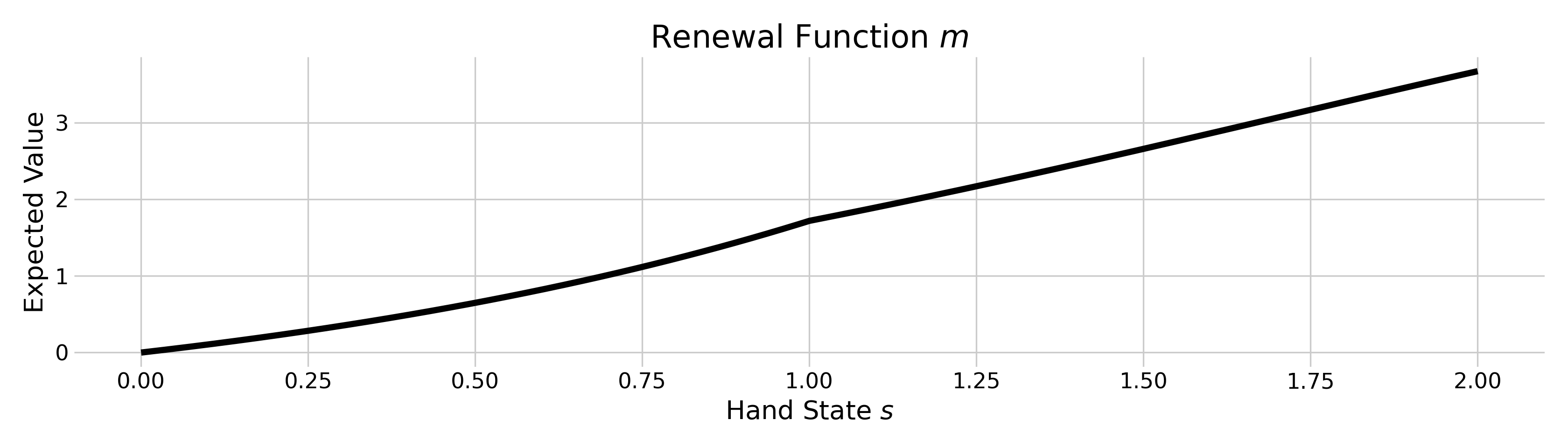
We can similarly derive \(m_1(s) \doteq m(s)\) for \(s \in [1, 2]\) by recalling that \(\alpha_1(s) = 1\) and \(\dot\alpha_1(s) = 0\) for all such \(s\). The renewal equation now takes the slightly different form $$m_1(s) = 1 + \int_0^s m_1(s - x) \, \mathrm{d}x = 1 + \int_0^1 m_1(s - x) \, \mathrm{d}x.$$ Note that (a) the first term reduces to unity, and (b) the bounds of integration preclude the interval \([1, s]\) since the measure is constant over that interval. Applying exactly the same process as before now yields the ODE $$\dot{m}_1(s) = m(s) - m(s - 1) = m_1(s) - m_0(s - 1),$$ where the second equality exploits the fact that \(m(s-1) = m_0(s-1)\) for all \(s \in [1, 2]\) since \(s - 1\) will lie in the former solution's domain. Multiplying both sides by the integrating factor \(e^{-s}\) gives \(e^{-s} [\dot{m}_1(s) - m_1(s)] = e^{-s} m_0(s - 1) = e^{-s} - e^{-1}\) which, after recognising that \(e^{-s} [\dot{m}_1(s) - m_1(s)] = \nabla_s e^{-s} m_1(s)\), can be integrated over \([1, s]\) to yield the solution $$\begin{aligned}m_1(s) &= e^s + e^{s-1} (1 - s) - 1, \\ &= m_0(s) + e^{s-1} (1 - s).\end{aligned}$$ It is interesting to note how the solution \(m_1\) comprises \(m_0\) plus a residual term. Indeed, this recursive pattern continues as \(s \to \infty\) as we'll prove next.

The General Case

In order to understand the general behaviour of \(m(s)\) we first need to identify a candidate form that we can verify. As it turns out, such a solution of the renewal equation does indeed exist and is given precisely by $$m(s) + 1 = \sum_{k=0}^{\lfloor s \rfloor} \frac{1}{k!} e^{s - k} (k - s)^k.$$ One need only look at the previous two solutions, and the solution for \(s \in [2, 3]\) (see below), to recognise the pattern. It remains only to formally prove this claim.

Let \(g_k(s) \doteq \frac{1}{k!} e^{s-k}(k-s)^k\) denote a series of functions for integer \(k \geq 0\), such that the proposed solution may be expressed as \(m(s) + 1 = \sum_{k=0}^{\lfloor s \rfloor} g_k(s)\). To prove that this is valid, we must verify that it satisfies the ODE \(\dot{m}(s) = m(s) - m(s-1)\) for all \(s \geq 0\) with boundary condition \(m(0) = 0\). The latter is clearly true since \(g_0(s) = 1\). On the former, let's first take derivatives with respect to \(s\) to get \(\dot{g}_k(s) = \frac{s}{s-k} g_k(s)\) and thus \(\dot{m}(s) = \sum_{k=0}^{\lfloor s \rfloor} \frac{s}{s-k} g_k(s)\). Substituting into the original ODE and grouping terms according to the arguments of \(g_k\) leads to $$\sum_{k=0}^{\lfloor s \rfloor} \frac{k}{k-s} g_k(s) = \sum_{k=0}^{\lfloor s \rfloor - 1} g_k(s - 1).$$ To prove that this equality holds, note that \(g_{k-1}(s-1) = \frac{k}{k-t} g_k(s-1)\) for all \(k \geq 1\), allowing us to express the second summation as \(\sum_{k=1}^{\lfloor s \rfloor} \frac{k}{k-t} g_k(s - 1)\). Since the first term (i.e. for \(k=0\)) of the first summation is necessarily zero, and \(s \geq 0\) was taken arbitrarily, we have our desired result, albeit rather unwieldy.

Limits and Approximations

The (closed-form!) expression for the renewal function is very convenient, but evaluating it becomes numerically unstable even for rather modest \(s \gtrsim 25\). This is in spite of the fact that \(g_k(s) \to 0\) as \(k \to \infty\). We may therefore ask whether reasonable approximations exist that don't involve variable summation or factorials, especially for large thresholds \(s\), for which we turn to the fundamental result in renewal theory.

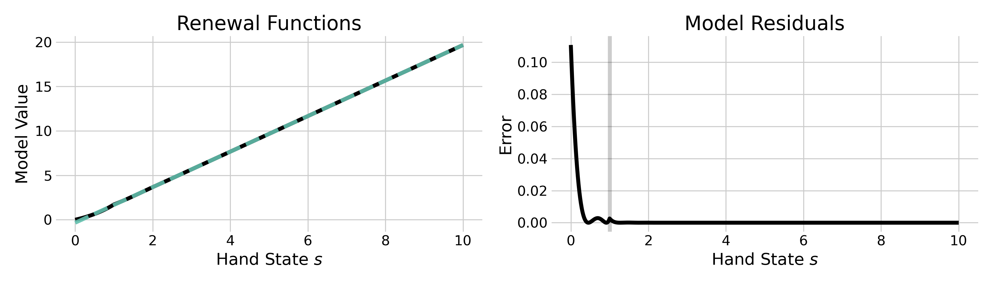
The elementary renewal theorem states that the long-run average rate of arrivals tends to \(\mu^{-1}\) over time, where \(\mu \doteq \mathbb{E}[X_1] = 2^{-1}\). More formally, it asserts that $$\lim_{s\to\infty} \frac{m(s)}{s} = \frac{1}{\mu},$$ for which a proof can be found in Grimmett and Stirzaker.^[2] With this in mind, we'll assume that \(m(s)\) can be approximated by a linear function with growth rate \(\mu^{-1}\) when \(s\) is large: $$\tilde{m}(s) \doteq 2s + c,$$ where \(\lim_{s\to\infty} \tilde{m}(s) = \mu^{-1}\) as intended. The appropriate offset \(c\) can then identified numerically using mean squared error under a uniform sampling assumption, leading to a value \(c \approx -3^{-1}\). As we can see from the figure above, the model residuals are quite poor for \(s \in [0, 1]\), but reduce quickly as the threshold grows. We'll make use of this approximation in the following section to simplify our analysis, but pay close attention to region in which it is valid.

Strategic Sums and Residual Life

At this point you would be forgiven for asking why we've spent so much time solving ODEs just to characterise the renewal function when our real interest lies in the distribution of \(S_{N(\tau) + 1}\). Maybe you feel like we should have just stuck to our guns and waded through subtlety to find an expression for \(P(S_{k + 1} \leq s \mid N(\tau) = k)\). Well, if you're still here, your patience has paid off... now we get to the good bit!

A key result of renewal theory states that, for any locally bounded function \(f : [0, \infty) \to \R\), the unique (locally bounded) solution to the renewal equation \(u = f + u * \alpha_1\) is given by \(u = f + f * m\), where \((a * b)(t) \doteq \int_0^t a(t - x) \, \mathrm{d}b(x)\) for suitable functions \(a\) and \(b\).^[b] This beautiful result, whose proof can be shown via an application of Laplace transforms (see box below), allows us to exploit the lengthy analysis of the renewal function to avoid solving recursive expressions every time we wish to understand (suitably-defined) functions such as \(f\).^[c] It thus remains only to find a suitable \(f\) such that we might recover the CDF of our terminal hand \(P(S_{N(\tau) + 1} \leq s)\).

Let us first define \(\sigma_\tau(s) \doteq P(S_{N(\tau) + 1} \leq s)\) and \(\nu_\tau(r) \doteq P(R(\tau) \leq r)\), where the latter is the CDF for the residual/excess life \(R(\tau) \doteq S_{N(\tau) + 1} - \tau\) at the stopping threshold \(\tau\). The quantity \(R(\tau)\) describes the excess compared with our last hand and thus fully characterises the probabilistic behaviour of \(S_{N(\tau) + 1}\). Concretely, the two CDFs are related by the translation \(\sigma_\tau(s) = \nu_\tau(s - \tau)\), with \(\nu_\tau\) satisfying the integral equation $$\nu_\tau(r) = \alpha_1(\tau + r) - \int_0^\tau [1 - \alpha_1(\tau + r - s)] \, \mathrm{d}m(s).$$ In other words, \(\nu_\tau(r)\) satisfies a renewal-type equation for which the corresponding function \(f\) is given by \(r \mapsto \alpha_1(\tau + r)\); see Grimmett and Stirzaker^[2] for a much more detailed exposition. We can now solve this directly, though, as before, we need to pay close attention to the domains of integration!

Let's consider the case where \(0 < \tau \leq 1\) such that \(m(\tau) = e^\tau - 1\). There are now three regions in the domain of the target distribution function that we must examine: \((0 \leq r \leq 1 - \tau)\), \((1 - \tau < r \leq 1)\) and \((r > 1)\). The last case is simple since \(\tau \leq S_{N(\tau) + 1} \leq \tau + 1\) almost surely, and thus \(P(R(\tau) > 1) = 0\). In the first case, we have that \(\alpha_1(\tau + r) = \tau + r\) and so we can express the above integral relation as $$\nu_\tau(r) = \tau + r - \int_0^\tau [1 + s - \tau - r] \, \dot{m}(s) \, \mathrm{d}s.$$ Evaluating \(\dot{m}\), substituting into the integral and solving yields \(\nu_\tau(r) = e^\tau r\). In the final case, where \(1 < \tau + r \leq 1 + \tau\), the integral is a bit more subtle. While it is certainly clear that \(\alpha_1(\tau + r) = 1\), the translated values \(\alpha_1(\tau + r - s)\) exhibit a second-order discontinuity at \(\tilde{s} = \tau + r - 1\) wherein \(\alpha_1(\tau + r - s') = 1\) for all \(s' \in [0, \tilde{s}]\). The renewal-type equation thus reduces to $$\nu_\tau(r) = 1 - \int_{\tau + r - 1}^\tau [1 + s - \tau - r] \, e^s \, \mathrm{d}s,$$ which further resolves to \(\nu_\tau(r) = e^\tau r - e^{\tau+r-1} + 1\). Combining these results, we have that, for \(0 \leq \tau \leq 1\), the CDF of the stopped sum is given by the piecewise function $$\sigma_\tau(\tau + r) \equiv \nu_\tau(r) = \begin{cases} 0 &\textrm{for } r < 0, \\ e^\tau r &\textrm{for } 0 \leq r \leq 1 - \tau, \\ e^\tau r - e^{\tau+r-1} + 1 &\textrm{for } 1 - \tau < r \leq 1, \\ 1 &\textrm{for } r > 1.\end{cases}$$

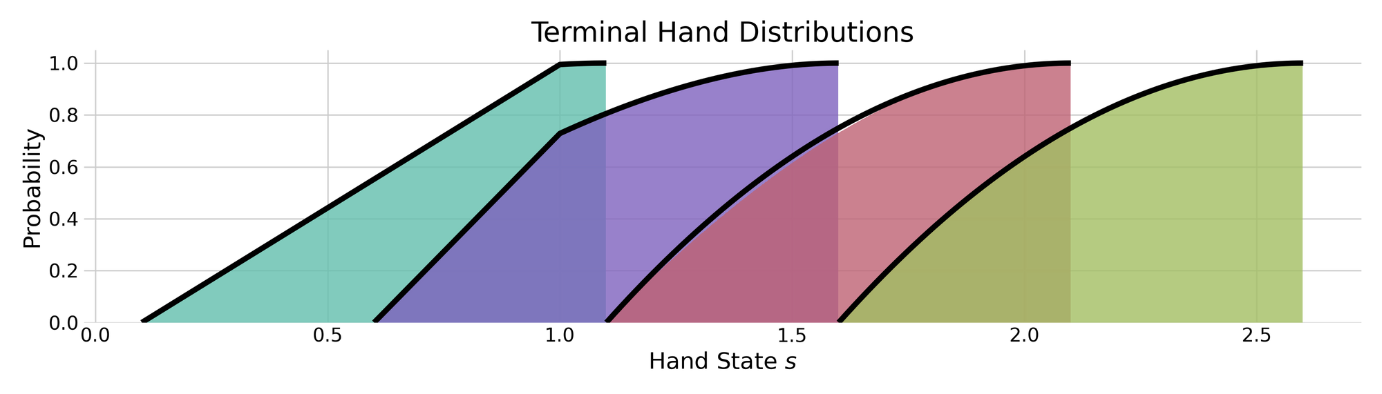
As with the analysis of the renewal function, we can extend these results to stopping times \(\tau > 1\), but in so doing we trade one complication for another. While we need only consider a single region in this case — i.e. \(\tau \leq s \leq \tau + 1\) wherein \(\alpha_1(s) = 1\) — the integral itself is significantly more complicated to evaluate. The reason is that \(\dot{m}(x)\) involves variable summation as well as integrals over maps of the form \(x \mapsto x g_k(x)\) and \(x \mapsto g_k(x)\) which involve factorial, exponential and quadratic terms in their solution. While we could proceed anyway, I favour a more pragmatic approach!

Limits and Approximations (again)

Rather than compute the exact solution using the renewal function \(m\), we're going to make use of our linear estimator \(\tilde{m}\) — derived from the elementary renewal theorem — to form an approximate measure \(\tilde{\nu}(r)\). Solving for this measure is dramatically simpler than \(\nu_\tau(r)\), and still yields an accurate estimate when compared with simulated results; see figure above. Skipping the routine derivation, we arrive at the wonderfully simply conclusion that $$\tilde{\nu}(r) = \begin{cases} 0 &\textrm{for } r < 0, \\ 1 - (r - 1)^2 &\textrm{for } 0 \leq r \leq 1, \\ 1 &\textrm{for } r > 1,\end{cases}$$ which is valid for all \(\tau \geq 1\). As you can see from the diagram above, this limit-based estimate exhibits significant errors for \(\tau\) close to 1, but grows increasingly accurate as the stopping threshold grows. The reason is that boundary effects near the second-order discontinuity in \(\alpha_1\) have a bearing on the solution only for \(\tau \in [1, 2]\), but the influence of this effect decreases rapidly. Since we've already spent some time on this topic, I leave it to you to find a better solution!^[d]

Optimality

As we know, the goal in continuous blackjack is (broadly speaking) to maximise your terminal hand without exceeding the upper limit \(\theta\). To model this, we introduced the notion of a stopping threshold \(\tau\) over which we commit to stop drawing new samples from the deck, and hold firm with the hand \(S_{N(\tau) + 1}\). The objective can thus be stated as the stochastic optimisation problem $$\tau^\star[u] \doteq \argmax_{\tau \in [0, \theta)} \left\{f(\tau) \doteq \mathbb{E}[u(\tau, S_{N(\tau) + 1})] = \int_\tau^{\tau + 1} u(\tau, s) \, \mathrm{d}\sigma_\tau(s)\right\}$$ for payoff functions for the form $$u \in \mathcal{U} \doteq \{u(\tau, s) = \mathbb{1}(s \leq \theta) \cdot g(\tau, s) + \mathbb{1}(s > \theta) \cdot h(\tau, s) : g\in\mathcal{G}, h\in\mathcal{H}\},$$ where the sets \(\mathcal{G}\) and \(\mathcal{H}\) comprise the absolutely integrable^[e] functions that are reward/risk compatible, respectively. The latter constraints require that all functions \(g\in\mathcal{G}\) be non-decreasing in \(s\) over the domain \((\infty, \theta]\), and that all functions \(h \in \mathcal{H}\) be non-positive and non-increasing for \(s \in (\theta, \infty)\). Together with absolute integrability, these ensure that \(f(\tau)\) is well-defined and yields intuitive results for the game being played.

It's worth noting here that the optimal stopping map \(\tau^\star : \mathcal{U} \to \mathfrak{B}((\infty, \theta))\) is expressed as a functional between the set of payoff functions \(\mathcal{U}\) and the Borel subsets of valid thresholds. For brevity, we will usually abuse notation by writing \(\tau^\star[g, h]\) with no loss of generality. Now, while the constraints on \(\mathcal{U}\) guarantee that \(f\) is finite, the set \(\tau^\star[u]\) may well be empty if the maximum isn't attained. This may seem like a technicality that can be avoided by replacing \(\max\) with \(\sup\), but we must ask ourselves what it would mean in the real world to roll out such a strategy. For example, functions of the form \(f(\tau) = \mathbb{1}(\tau < x) \cdot \tau - \mathbb{1}(\tau = x) \cdot T\) for large \(T < \infty\) might suggest stopping at some \(x - \varepsilon\) for small \(\varepsilon > 0\), but the induced distribution of \(S_{N(x - \varepsilon) + 1}\) may very well have extremely undesirable properties with regards to risk. Personally, I find it much more conceptually meaningful to require that the expected payoff under an optimal strategy actually exists, and thus avoid these concerns entirely.

The General Case

The structure we've imposed on payoff functions and their risk/reward components allows us to make one particularly useful observation: any and all optimal thresholds are guaranteed to lie in the interval \(\mathcal{T} \doteq [(\theta - 1)_+, \theta)\) for all \(u \in \mathcal{U}\) with monotonically increasing \(g\) over \(s \in (\infty, \theta]\). Further, in the case where \(g\) only satisfies the original non-decreasing condition, then we may still restrict our attention only to this interval since \(\tau[u] \cap \mathcal{T} \ne \emptyset\) and all elements of \(\tau^\star[u]\) yield the same payoff in expectation;^[f] i.e. \(f(\tau^\star[u])\) is either empty or a singleton set. You should spend a little time contemplating why this is true.

An immediate consequence of the above result is that we need only search over thresholds \(\tau \in \mathcal{T}\) during optimisation as opposed to the whole space. This reduces the complexity of the problem, especially when \(\theta\) is large or numerical methods are being used. We can also re-express the "optimand" using the structure of \(u\) directly, yielding $$f(\tau) = \int_\tau^\theta g(\tau, s) \, \mathrm{d}\sigma_\tau(s) + \int_\theta^{\tau + 1} h(\tau, s) \, \mathrm{d}\sigma_\tau(s).$$ In the case where \(f\) is differentiable, we can also write a first-order optimality condition $$\begin{aligned}0 = & \,\, \dot\sigma_\tau(\tau+1) h(\tau, \tau+1) - \dot\sigma_\tau(\tau) g(\tau, \tau) \\ &+ \int_\tau^\theta \dot\sigma_\tau(s) \nabla_\tau g(\tau, s) + g(\tau, s) \nabla_\tau \dot\sigma_\tau(s) \, \mathrm{d}s \\ &+ \int_\theta^{\tau+1} \dot\sigma_\tau(s) \nabla_\tau h(\tau, s) + h(\tau, s) \nabla_\tau \dot\sigma_\tau(s) \, \mathrm{d}s, \end{aligned}$$ wherein the right hand side should be evaluated at \(\tau = \tau^\star\). Now, this may look pretty unwieldy, but many of these terms drop out for common payoff functions. For example, many components \(g\) and \(h\) have no explicit dependence on the threshold itself, only on the terminal hand \(s\), as we shall see in the next section.

Partitioning on \(\theta\)

There are two key cases that we might consider given our previous analysis: \(\theta \leq 1\), for which we use the exact measure \(\sigma_\tau\); and \(\theta > 1\), for which we replace \(\sigma_\tau\) with the approximate measure \(\tilde\sigma\). Each variant leads to it's own specialisation of the first-order condition. In the former case, we have \(\dot\sigma_\tau(s) = e^\tau\) and \(\nabla_\tau \dot\sigma_\tau(s) = e^\tau\) which implies that all terms have an exponential factor contributing only non-finite solutions. We can safely drop these, and write (in short-hand, for brevity) $$g - h - \int_\tau^\theta \nabla_\tau g + g \, \mathrm{d}s - \int_\theta^{\tau+1} \nabla_\tau h + h \, \mathrm{d}s = 0.$$ In the latter case, we have instead \(\dot{\tilde\sigma}(s) = -2(1 + \tau - s)\) and \(\nabla_\tau \dot{\tilde\sigma}(s) = -2\), and the optimality condition reduces to $$g - \int_\tau^\theta (1 + \tau - s)\nabla_\tau g + g \, \mathrm{d}s - \int_\theta^{\tau+1} (1 + \tau - s)\nabla_\tau h + h \, \mathrm{d}s = 0.$$ In this case we don't have any exponential terms, but we do find that many terms cancel and drop out — excellent!

Risk-Neutral Payoffs

The first class of payoff functions that we'll consider are of the form \(u(\tau, s) = \mathbb{1}(s \leq \theta) \cdot g(\tau, s)\) wherein the risk term is identically zero. We denote this class by \(\mathcal{U}_\textrm{N} \subset \mathcal{U}\) for which the goal, given some \(g \in \mathcal{G}\), is to identify an element of the optimal stopping set \(\tau^\star[g, 0]\). Payoffs of this form don't explicitly penalise the player for going bust, but they do allow us to design incentives around how close one should get to \(\theta\). We thus refer to this class as risk-neutral because, assuming there is no fee for playing the game, there is also no risk associated with a bad hand. While this is not a particularly natural set of payoffs for a gamling problem, it is informative to study.

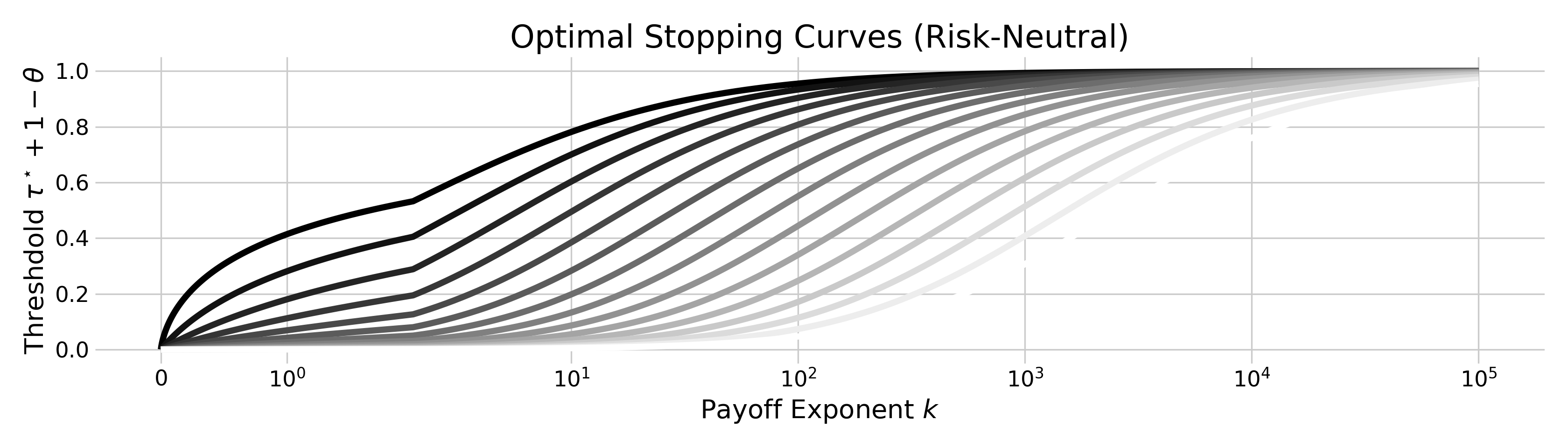
As a concrete example, consider the polynomial component function \(g(\tau, s) = s^k\) for given \(k \geq 0\). Plugging this equation into our optimality condition for \(\theta = 1\) yields the \((k+1)\)-th order polynomial equation for \(\tau^\star\), $$\tau^{k+1} + (k+1) \tau^k - 1 = 0.$$ Finding analytical solutions to this for \(k > 2\) or non-integer \(k\) gets tricky pretty quickly. Fortunately, root finding algorithms such as Brent's method make light work of it, especially since we can constrain our search space to points in \([0, 1]\); see the illustration above. We can perform a similar computation for the case where \(\theta > 1\) by using \(\tilde\sigma\), in which case we arrive at the fascinating conclusion that \(\tau^\star\) satisfies the analogous relation $$\tau^{k+1} + (k+1) \tau^k - \theta^{k+1} = 0;$$ I find this equivalence to be really quite miraculous! As you can see from the diagram above, the corresponding map \(\tau^\star[s \mapsto s^k, 0]\) has a unique value and is monotonically increasing in the exponent. We also observe that each curve is bounded above by all preceding cases in which the limit \(\theta\) is smaller.

Risk-Sensitive Payoffs

In the previous section we examined the case where \(h(\tau, s) = 0\) for all inputs, in which case any \(g > 0\) is gauranteed to yield positive expected returns and you are always incentivized to play the game. We will not look at what happens when there is an explicit penalty on losing. To be specific, we'll analyse payoffs of the form $$u(\tau, s) = \mathbb{1}(s \leq \theta) \cdot s^k - \mathbb{1}(s > \theta) \cdot s^m.$$ While this is by no means the only choice we could make, it will serve our purposes. Indeed, until we consider the multi-agent case in the next article, many of the conclusions we draw here are merely to gain foundational intuition.

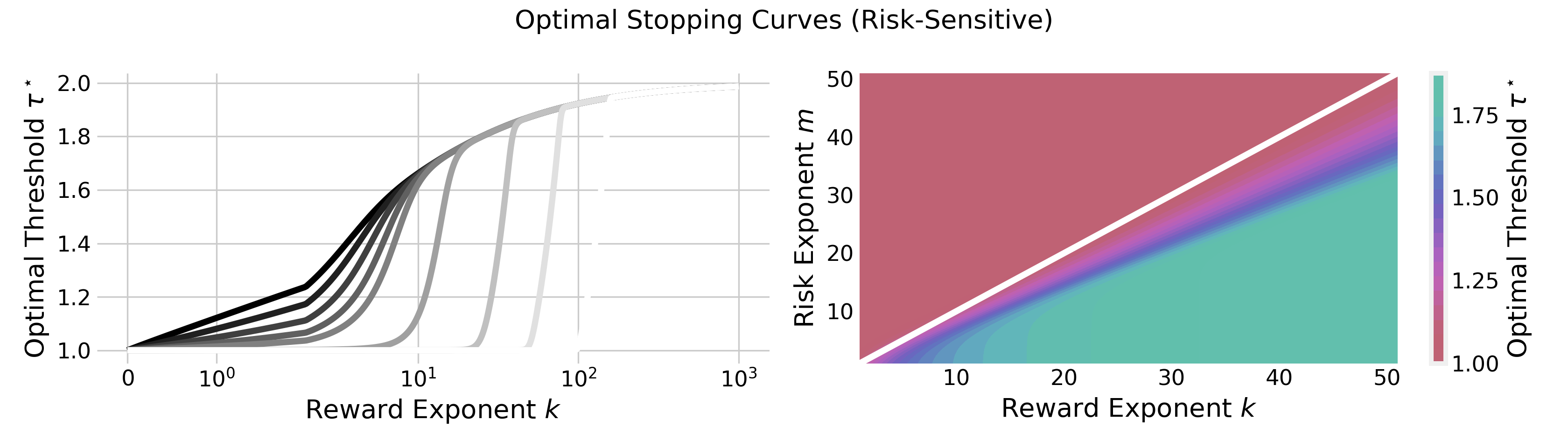
Since we previously saw that \(\sigma_\tau\) and \(\tilde\sigma\) gave rise to the same solution set, we'll just stick with the approximate measure for brevity, and set \(\theta = 2\). Following the same procedure as before, we arrive at the slightly more complicated optimality condition $$\tau^k + \frac{\tau^{k+1} - \theta^{k+1}}{k+1} + \frac{(\tau+1)^{m+1} - \theta^{m+1}}{m+1} = 0.$$ Again, we don't have much chance solving this analytically, but numerical methods can help us there; the result is illustrated in the figure above. In this case we see that whenever \(m > k\), the optimal solution is to stop at exactly \(\theta - 1\). This makes perfect sense, since stopping at \(\theta - 1\) guarantees that no hand ever exceeds the limit, and no penalty is received. Indeed, in absence of any competition, I claim that a rational player would be totally justified in playing this strategy, especially in finitely repeated settings. Conversely, when \(m < k\), we observe similar monotonicity properties as before, but with increasingly sharp gradients as \(m\) grows larger. This also aligns with intuition — when the positive payoff outweighs the negative, we're more incentivised to play risky.

Well... that ended up a little longer than anticipated. We covered hands and their distributions, renewal processes and their dynamics, and optimal stopping problems therein. Hopefully it's given you some idea of how to tackle problems of this form; I know that I've certainly learnt a lot from the process. As I mentioned at the start, the plan is to write subsequent articles about other aspects of the problem, so be sure to check in for that. Otherwise, I sincerely hope you enjoyed.

Notes

a. As a concrete example of such a process, consider the case in which we have a choice between two different decks: one with larger values, and the other with smaller values. Naturally, as our hand grows, we might shift from the former to the latter. This of course breaks the IID assumption, but does yield an adapted Markov process since \(X_{n+1}\) only depends on \(S_n\); we may consider this in follow-up articles.
b. The operator \(*\) defined here is of a convolutional flavour, but it is not the same as the traditional convolution. In this case, the latter argument must be defined such that we have a well-formed Lebesgue-Stieltjes integral; e.g. of bounded variation and right-continuous.
c. The renewal function \(m\) fully characterises the renewal process by "carrying" the sequential/convolutional information. The operation \(f \mapsto f + f * m\) then acts as to "embed" this information in the context of a function of interest \(f\).
d. One approach to this would be to define \(\tilde{m}\) as a piecewise function, with the true solution on \(t \in [0, 1]\) and the linear approximation on \(t \in (1, \infty]\). This would form a much better estimate, but leads to some rather tedious integral analysis. Good luck, and feel free to send me your conclusions!
e. Recall that a function \(f : \Omega \to \R\) is said to be integrable with respect to a measure \(\mu\) if \(\int\lvert f(x) \rvert \, \mathrm{d}\mu(x) < +\infty\). Since the RN derivative \(\dot\sigma_\tau\) is well-defined for all valid \(\tau\), we have that absolutely integrability implies \(\sigma_\tau\)-integrability which suits our purposes.
f. Note that this would not necessarily hold if we were to explicitly consider additional statistics such as variance.

Bibliography

1. Marengo, J.E., Farnsworth, D.L. and Stefanic, L. A Geometric Derivation of the Irwin-Hall Distribution. International Journal of Mathematics and Mathematical Sciences (2017).
2. Grimmett, G., and Stirzaker, D. Probability and Random Processes. Oxford University Press (2020).
3. Herschkorn, S.J., and BSI Problems Group. Continuous Blackjack: 11287. The American Mathematical Monthly (2008).